Differential Equation Solver

What Is a Differential Equation Solver?

A differential equation solver is a tool that finds the function or functions satisfying an equation that relates a function to its derivatives. Unlike algebraic equations where you solve for a number, differential equations are solved for a function — typically written as y(x) or y(t) — that satisfies the given relationship between the function and its rate of change.

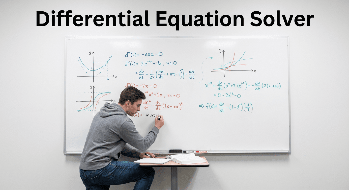
Differential equations are the mathematical backbone of physics, engineering, biology, economics, and nearly every technical field. They describe how systems change over time or space: the motion of a pendulum, the cooling of an object, the spread of a disease, the flow of electrical current, or the growth of a population. Being able to solve a differential equation means you can predict how a system behaves given its current state — which is precisely what this diff eq solver does instantly.

This AI-powered ODE solver handles first-order, second-order, and higher-order ordinary differential equations, as well as separable, linear, exact, and Bernoulli equations. It can solve general solutions, particular solutions given initial conditions, and provide full step-by-step working. It is the equivalent of having a diff eq calculator that also explains every method it uses.

How the Differential Equation Solver Works

Enter Your Equation

Type your differential equation into the input field using standard notation. You can write dy/dx for the first derivative, y' or y'' for shorthand notation, or d²y/dx² for explicit second derivative notation. The solver accepts a wide range of input formats so you do not need to reformat your equation before submitting. Examples: dy/dx = 2x + y, y'' + 3y' + 2y = 0, or dx/dt = x - y, dy/dt = x + y for a system.

Specify Type and Conditions

Select the equation type from the dropdown to help the solver apply the correct method from the start. If you have initial conditions — values of y or its derivatives at a specific point — enter them in the Initial Conditions field using notation like y(0) = 1, y'(0) = 0. Then choose what you need: a general solution with arbitrary constants, a particular solution with constants determined by your initial data, a full step-by-step walkthrough, or a graph description that explains the qualitative behavior of the solution.

Get Step-by-Step Solution

Click Solve Equation and the AI differential equations calculator processes your input and returns a complete mathematical solution. The step-by-step mode names the solution method, shows each algebraic manipulation, derives the integrating factor or characteristic equation where needed, integrates, and applies initial conditions if provided. You can continue the conversation to ask follow-up questions, request a different method, or check specific steps.

Types of Differential Equations

First-Order ODEs

A first-order ordinary differential equation involves only the first derivative of the unknown function. The general form is dy/dx = f(x, y). First-order ODEs are the most common type encountered in introductory calculus and applied mathematics. They model exponential growth and decay, Newton's law of cooling, simple electrical circuits, and mixing problems. Solution methods depend on the structure of f(x, y) — separable equations, linear equations, exact equations, and Bernoulli equations each have distinct techniques.

Second-Order ODEs

Second-order ODEs involve the second derivative y'' and arise in mechanical vibrations, electrical RLC circuits, and structural analysis. The standard form is ay'' + by' + cy = g(x). When g(x) = 0, the equation is homogeneous and solved using the characteristic equation. When g(x) is nonzero, the equation is non-homogeneous and requires a particular solution found by undetermined coefficients or variation of parameters added to the homogeneous solution.

Separable Equations

A separable differential equation can be written so that all terms involving y are on one side and all terms involving x are on the other: g(y)dy = f(x)dx. This structure allows direct integration of both sides independently. Separable equations are among the simplest to solve analytically and are a foundational technique in any differential equations course. Population growth models, radioactive decay, and terminal velocity problems typically produce separable ODEs.

Linear Equations

A first-order linear ODE has the form dy/dx + P(x)y = Q(x). The standard solution technique multiplies both sides by an integrating factor μ(x) = e^(∫P(x)dx), which transforms the left side into the derivative of a product. After integration, dividing by the integrating factor yields the general solution. Linear equations model circuits with varying voltage, drag forces, and mixing tanks — systems where the response is proportional to the input.

Exact Equations

An exact differential equation is one where M(x,y)dx + N(x,y)dy = 0 and the partial derivative of M with respect to y equals the partial derivative of N with respect to x. When this condition holds, the equation is the total differential of some function F(x,y), and the solution is F(x,y) = C. If the exactness condition is not met, an integrating factor can sometimes be found to make the equation exact.

Solution Methods

Separation of Variables

Separation of variables is the most direct solution method for separable ODEs. The equation is rearranged to isolate the y terms on the left and x terms on the right, then both sides are integrated. The technique produces a general solution containing one arbitrary constant for first-order equations. If initial conditions are provided, substituting them eliminates the constant and gives the particular solution unique to the initial value problem.

Integrating Factors

The integrating factor method applies to first-order linear ODEs of the form dy/dx + P(x)y = Q(x). The integrating factor μ(x) = e^(∫P(x)dx) is calculated first, then the entire equation is multiplied through by μ(x). The left side becomes d/dx[μ(x)y], which integrates directly. The right side ∫μ(x)Q(x)dx may require standard integration techniques. This method is reliable for any first-order linear ODE regardless of the functions P(x) and Q(x).

Characteristic Equation

For second-order homogeneous linear ODEs with constant coefficients ay'' + by' + cy = 0, the characteristic equation ar² + br + c = 0 is formed by substituting the trial solution y = e^(rx). Solving the characteristic equation gives two roots r₁ and r₂. If the roots are real and distinct, the general solution is y = C₁e^(r₁x) + C₂e^(r₂x). Repeated roots yield y = (C₁ + C₂x)e^(rx). Complex conjugate roots α ± βi produce y = e^(αx)(C₁cos(βx) + C₂sin(βx)).

Variation of Parameters

Variation of parameters finds a particular solution to a non-homogeneous ODE by replacing the constants in the homogeneous solution with functions. For ay'' + by' + cy = g(x), the homogeneous solution y_h = C₁y₁ + C₂y₂ is found first. The particular solution is then assumed to be y_p = u₁(x)y₁ + u₂(x)y₂ where u₁' and u₂' are determined by a system of two equations derived from the Wronskian. This method works for any continuous g(x), making it more general than undetermined coefficients.

Differential Equation Examples

Example 1 - First-Order Separable

Example 2 - Second-Order Homogeneous

Who Uses a Differential Equation Solver?

Undergraduate and graduate students in mathematics, physics, engineering, and biology use an ODE solver to check homework, verify exam practice problems, and understand unfamiliar solution techniques. When a diff eq calculator shows each step, students learn the method rather than just seeing the answer.

Engineers use differential equation solvers to prototype solutions before implementing numerical methods in software. Physicists model wave equations, quantum systems, and orbital mechanics. Data scientists and economists model dynamic systems in finance and resource allocation. For all these users, a differential equations calculator free of cost and accessible from any browser is an essential working tool.

If you also need help with related mathematical problems, the free AI math solver covers algebra, calculus, and more. For statistical analysis alongside your differential equations work, the AI statistics solver handles probability, distributions, and hypothesis testing. If you are working on physics problems that involve ODEs, the free AI physics solver provides context-specific solutions. For broader academic support, the AI homework helper covers multiple subjects simultaneously.

Differential Equation Solver vs Other Math Tools

A general-purpose math solver handles a wide range of algebraic and computational problems but may not apply the specialized techniques required for ODEs — such as finding integrating factors, forming characteristic equations, or using variation of parameters. This differential equation solver is purpose-built for ODE problems and applies the correct mathematical method based on the equation type you specify.

The compound inequalities solver and the multi-step equation solver work on static algebraic expressions without derivatives. Differential equations require a fundamentally different approach — identifying the equation class, choosing the solution method, performing integration, and applying constraints from initial conditions. This tool is designed specifically for that workflow. For a broader overview of AI math tools, see the AI math solvers hub.

Frequently Asked Questions